Visualizing Eigenvalue Distributions through Matrix Evolution

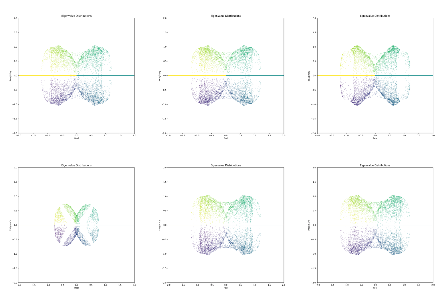
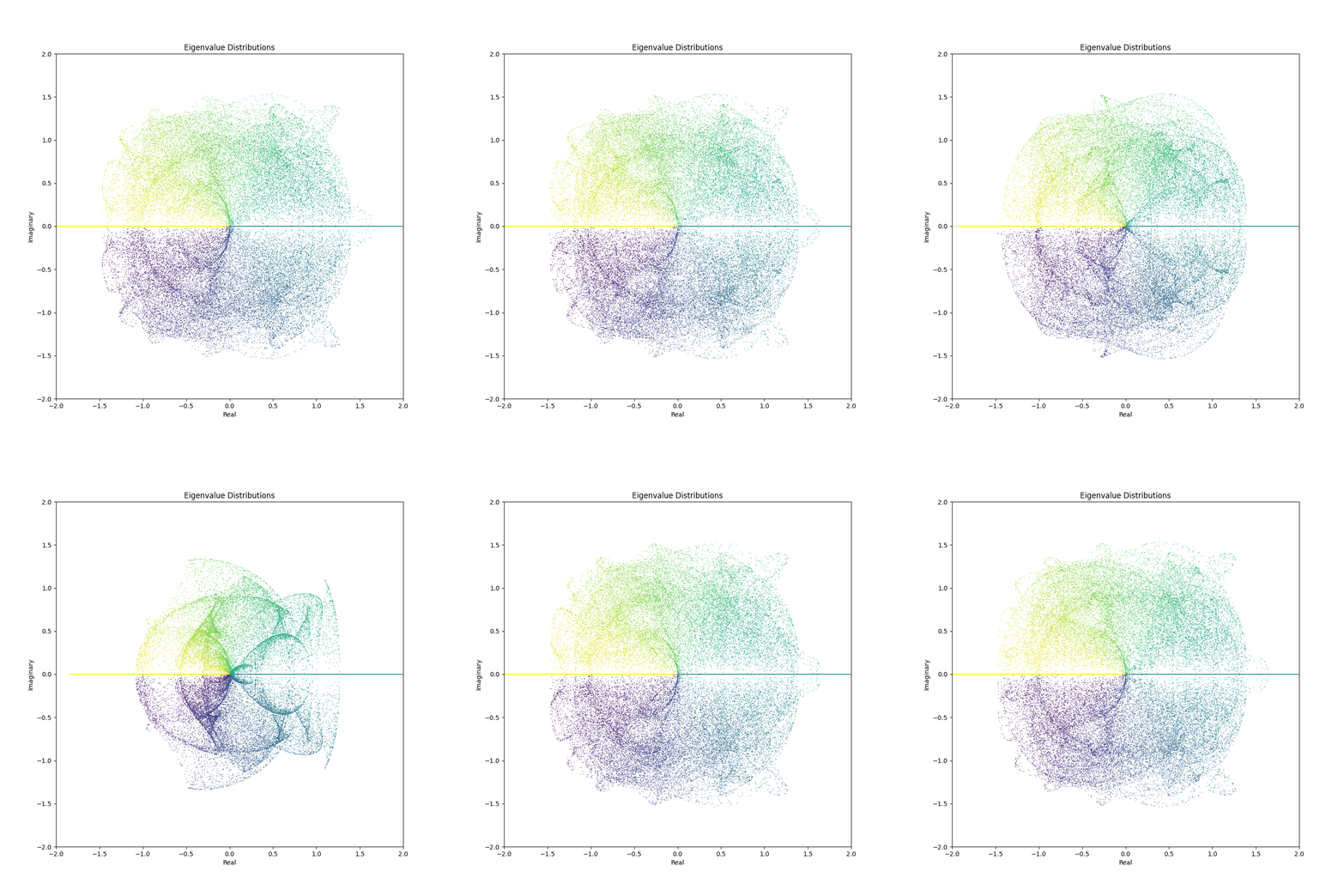
In a delightful dive into the visual world of matrices and eigenvalues, I stumbled upon a Twitter post showcasing a fascinating visualization of eigenvalue distributions evolving over a parameter space. Intrigued by the aesthetics and the mathematical underpinnings, I decided to recreate and explore this visual journey using Python.

Unveiling the Mathematics

The process of visualizing the eigenvalue distributions involves three primary steps:

1. Matrix Generation: We start by defining a matrix whose elements are governed by mathematical functions and parameters. The original post used a specific 6x6 matrix, but the beauty of this exploration lies in its versatility. We can craft different matrix generation functions to unveil unique visual patterns.

2. Eigenvalue Calculation: For each matrix instance, we compute its eigenvalues. Eigenvalues reveal fascinating properties about the linear transformations represented by the matrices. They are complex numbers and can be visualized in a 2D space with real and imaginary parts as coordinates.

3. Parameter Evolution: A parameter within the matrix generation function is evolved over a range, which, in turn, alters the matrix and its eigenvalues. Observing how the eigenvalue distributions morph as the parameter changes provides a captivating visual representation.

Diving into Code

Let’s delve into the coding part where we encapsulate the above steps into a function to animate the eigenvalue distributions.

Matrix Generation Function

We define a matrix generation function. In this example, a 3x3 matrix is generated using trigonometric functions and normally distributed random numbers.

import numpy as np

def harmonic_matrix(t1, t2, x):
    # Defining harmonic relationships
    harmonics_t1 = np.array([t1, 2*t1, 3*t1])
    harmonics_t2 = np.array([t2, 2*t2, 3*t2])
    
    # Creating a matrix using harmonic relationships
    matrix = np.array([
        [np.sin(harmonics_t1 * x), np.cos(harmonics_t2 * x), np.sin((harmonics_t1 + harmonics_t2) * x)],
        [np.cos(harmonics_t1 * x), np.sin(harmonics_t2 * x), np.cos((harmonics_t1 + harmonics_t2) * x)],
        [np.sin((harmonics_t1 - harmonics_t2) * x), np.cos((harmonics_t1 - harmonics_t2) * x), np.sin((harmonics_t1 + harmonics_t2) * x)]
    ])
    return matrix

Animation Function

We create a function to animate the eigenvalue distributions using Matplotlib. This function takes in the matrix generation function, a range for the evolving parameter, and other optional arguments.

import matplotlib.pyplot as plt
import matplotlib.animation as animation
from IPython.display import HTML

def animate_eigens(matrix_func, x_range=np.arange(-np.pi, np.pi, np.pi/10), sample_size=10000,
                   xylim=[-2, 2], filename=None):
    fig, ax = plt.subplots(figsize=(10,10))
    scat = ax.scatter([], [], s=1, c=[], cmap=plt.cm.viridis, edgecolors=None, linewidth=0)  # Changed colormap here

    def init():
        ax.set_xlim(xylim)
        ax.set_ylim(xylim)
        ax.set_xlabel('Real')
        ax.set_ylabel('Imaginary')
        ax.set_title('Eigenvalue Distributions')
        return scat,

    def update(frame):
        x = x_range[frame]
        eigenvalues = np.empty((0,))
        for _ in range(sample_size):
            t1, t2 = np.random.uniform(-np.pi, np.pi, 2)
            matrix = matrix_func(t1, t2, x)
            eigenvalues = np.append(eigenvalues, np.linalg.eigvals(matrix))
        scat.set_offsets(np.c_[eigenvalues.real, eigenvalues.imag])
        scat.set_array(np.angle(eigenvalues))  # Color by phase
        return scat,

    ani = animation.FuncAnimation(fig, update, frames=len(x_range), init_func=init, blit=True, repeat=False)
    if filename is not None:
        ani.save(filename, writer='imagemagick', fps=15)
    plt.close(fig)  # Close the figure to prevent displaying it inline
    return HTML(ani.to_html5_video())

# Generate and save the animation
animate_eigens(trigonometric_normal_matrix)

In the animate_eigens function, we iteratively generate matrices using the matrix_func, compute their eigenvalues, and update the scatter plot to reflect the evolving eigenvalue distributions.

Unfurling the Visuals

With the code snippets above, you can now generate mesmerizing animations depicting the evolution of eigenvalue distributions. Here are some GIFs created using different matrix generation functions and parameter ranges: (Insert GIFs here)

Feel free to tweak the matrix generation functions or come up with your own to unveil a myriad of visual patterns waiting to be discovered. The confluence of mathematics and aesthetics opens a door to endless explorations and visual delights.