Evolution Strategies as an alternative to Reinforcement Learning for Solving the Lost Sales Inventory Management Problem

Summary

We show how to use Evolution Strategies (ES) to train neural networks for managing inventory in lost sales problem.
ES can learn significantly smaller neural network architechtures in comparison to RL methods without much need for hyper-parameter optimization.

Introduction

Deep Reinforcement Learning (DRL) agents have recently demonstrated their potential for solving sequential decision-making problems in various domains, such as playing Atari and Alpha Go games. This suggests that DRL agents could also be used to solve sequential decision-making problems in inventory management. While exact algorithms solve small instances of these problems efficiently, they fail in solving bigger instances in a reasonable amount of time due to the curse of dimensionality. Hence, researchers have usually designed heuristics for solving bigger-scale problems using the structural properties of the problem. Designing heuristics requires significant specialized knowledge about the problem. In addition, researchers usually make simplifying assumptions about the problem to come up with these heuristics, which limits their application areas. Hence, learning heuristics for solving sequential decision-making problems in inventory management using DRL seems promising.

DRL methodologies are subclass policy and value function approximation methods for solving sequential decision-making problems modeled as a Markov Decision Process (MDP). Value function approximation methodologies estimate the value of being in a certain state, which then can be used in choosing the right action in that state. On the other hand, policy approximation aims at predicting the best action directly from the state. While the practice of using approximate policy or value functions in solving sequential inventory management problems has been around for a while, recently it has been shown to scale. Hence, DRL methods are arising as a promising direction to learn heuristics for solving sequential decision-making problems. The main advantage of these algorithms is that they can solve different sequential decisions making problems without significant domain knowledge. However, this generality comes at the increased computational cost for learning the policy or value function approximators. In addition, the currently available DRL methods are sample inefficient, computationally intensive, and require lots of hyper-parameter optimization.

Recently, it has been shown that it is possible to learn a DRL agent to solve the lost sales problem with decent performance on small scale problems. However, the current applications of the DRL to inventory management problems are computationally inefficient and require significant hyper-parameter optimization. In this post, we show that one can overcome these limitations of DRL by using Covariance Matrix Adaptation Evolution Strategies (CMA-ES) which is a subclass of Evolution Strategies. Evolutionary methods have been shown to be a competitive alternative to DRL methods in solving sequential decision-making problems. Salimans, et al. (2017) show that a simple variant of the Natural Evolution Strategies (NES) can achieve similar performance to the DRL methods on Atari and Mujoco environments. ES has several advantages over DRL methodologies. It is highly parallelizable, invariant to action frequency, and delayed rewards. In addition, the gradient-free nature of the ES makes optimization on non-differentiable objective functions and neural network outputs possible. We show that one can use the objective function of the problem rather than defining policy, value, and entropy costs.

In this post, we show how to use the CMA-ES as an alternative to the popular DRL techniques such as Q-learning and Policy Gradients and their variants for solving inventory management problems. In particular, we show how to train a policy network that decide on the number of products to order in each time-step of the lost sales problem without the need for hyper-parameter optimization.

The rest of this post is structured as follows. We first give an overview of the lost sales inventory management problem. Then, we show how to optimize the parameters of a two-layer neural network that decides on the number of products to be ordered at each step of the inventory management problem (referred to as environment). In addition, we show how to speed up the training procedure using parallel processing. Finally, we evaluate the performance of the trained neural networks and conclude the post by giving directions for future research directions.

Notes on implementation

The results presented in this post can be replicated using my Github repository. I explain the main parts of the training procedure in the following sections of this post.

Lost sales inventory management problem

The Lost Sales problem is one of the fundamental problems in the inventory management literature (Zipkin, 2008, Bijvank and Vis, 2011). In this post, we consider the standard lost sales inventory management problem with discrete time-steps and a single item. The demand and order quantities are assumed to be integer. The objective of the problem is to minimize the long-run average cost of the system, which consists of the lost sales and inventory holding costs. The inventory manager has to decide on order quantity $q_t $ to be ordered at the beginning of period $ t \in {1, 2, \dots, T } $ where $T$ is the horizon of the environment. The ordered products will arrive in $ l > 0 $ periods from period $t$ (in period $l+t $). Afterwards, the new set of products of size $q_{t-l} $ ordered in period $t-l$ arrive. The inventory level of the system is then increased by $I_t = I_{t-1} + q_{t-l+1}$ where $I_t$ is the inventory level of the system at period $t$. An arriving demand of size $d_t$ is satisfied if there is enough inventory on hand, otherwise $d_t - I_t$ of the arriving demand will be lost. Let $h$ and $p$ denote the inventory holding and backlog costs of the system. In this tutorial, we assume that inventory procurement costs are zero without loss of generality. The cost function in period $t$ can be written as: $$ \begin{equation*} C_t(S_t) = h[I_t]^+ + p[d_t - I_{t-1} - q_{t-l}]^+, \end{equation*} $$ where $S_t$ is the current state of the system consisting of the current on-hand inventory and order pipeline. The order pipeline at the end of period $t-1$ consists of $Q_{t-1} = \left( q_{t-l}, q_{t-l+1}, \dots, q_{t-1}, \right)$. $S_t$ can be fully specified using the order pipeline and on-hand inventory as: $$\begin{equation*} S_{t} = \left( q_{t-l} + I_{t-1}, q_{t-l+1}, \dots, q_{t-1} \right). \end{equation*} $$ We use $S_t$ as an input of our policy network.

Python Simulation of the lost sales problem

In this post, we use the python simulation of the lost sales problem for training the ES agents. The implementation of the environment can be found here. The lost sales environment can be initialized as follows using the arguments of the environment:

env = LostSalesEnv(demand_rate=args.demand_rate, lead_time=args.lead_time, horizon=args.horizon,
                       max_order_size=args.max_order_size, holding_cost=args.holding_cost,
                       shortage_cost=args.shortage_cost, track_demand=track_demand)

You can set the arguments of the environment in the config.py file here with the following set of parameters:

parser.add_argument("--demand_rate", default=5, type=float, help="demand rate")
parser.add_argument("--max_order_size", default=25, type=int, help="maximum order size")
parser.add_argument("--lead_time", default=2, type=int, help="lead time")
parser.add_argument("--shortage_cost", default=4, type=float, help="shortage cost of the system")
parser.add_argument("--holding_cost", default=1, type=float, help="holding cost of the system")
parser.add_argument("--horizon", default=int(5e2), type=int, help="number of simulation epochs")

Hueristic methods for solving lost sales problem

Researchers have proposed several heuristics in the literature of inventory management for solving the lost sales problem. Zipkin (2008) gives an overview of the most recent heuristics and their performance in solving different sets of small-scale lost-sales problems. His results show that Myopic2 is one of the best performing heuristics for solving the lost sales problem. In this post, we use the Myopic2 policy as a benchmark for comparing the performance of the learned heuristics. We also investigate how using the upper bounds from the Standard Vector Base Stock policy on the number of ordered products can impact the performance of the learning algorithm. The implementation of these policies can be found here.

Example problems

In order to show the performance of ES in training control agents for the lost sales problem we evaluate its performance in different settings.

Lost sales problem with Poisson demand distribution

We consider three different lost sales problems with Poisson demand distribution. The problems differ in their lead and are labeled as Eesy, Medium and hard.

Problem	holding cost	shortage cost	lead time	demand rate
Easy	1	4	2	5
Medium	1	4	4	5
Hard	1	4	16	5

Evolution Strategies (ES)

Evolution Strategy is a population based stochastic continuous optmization methodology. It is related to the familiy of evolutionary population based algorithms such as the Genetic Algorithm. ES has been traditionally used for optimizing lower dimensional poroblems. However, recent works demonstrate that evolutionary algorithms can be scaled to optimize neural networks with several million parameters. In this tutorial, we will treat the ES as a black-box optimizer. For further details on how does the internals of the optimizer works, you can visit [my], David Ha or lilian Wang blog post. The application of evolutionary algorithms for solving RL problem is not new. However, it was the work of Salimans that showed ES as a scalable alternative to the DRL based algorithms.

Training with ES consists of three main parts at each iteration of the training as shown in the following code snippet. First, we ask the ES optimizer for a new set of population parameters where the size of each individual in the population is equal to the number of parameters of the policy network. Then, we evaluate the performance of each individual (each policy network) in controlling the environment. Finally, we say the rewards or fitness back to the ES optimizer to update the internal parameters of the optimizer.

    esopt = ES(num_params=num_params, popsize=es_population_size)
    for epoch in range(1, number_of_training_epochs + 1):
        solutions = esopt.ask()
        # Get the rewards of each es individual 
        esopt.tell(rewards)

We use the ESModule defined below which is inherited from the torch.nn.Module in setting the parameters of the neural network that are sampled from the ES optimizer.

import torch


class ESModule(torch.nn.Module):

    def get_model_shapes(self):
        """
        returns the shapes of the model parameters
        """
        model_shapes = []
        for param in self.parameters():
            p = param.data.cpu().numpy()
            model_shapes.append(p.shape)
            param.requires_grad = False
        return model_shapes

    @property
    def model_shapes(self, ):
        return self.get_model_shapes()

    def set_model_params(self, flat_params):
        """
        Sets the current parametrs of the  neural network to the flat_params based on the model shapes
        """
        assert 
        model_shapes = self.model_shapes
        idx = 0

        for i, param in enumerate(self.parameters()):
            delta = np.product(model_shapes[i])
            block = flat_params[idx: idx + delta]
            block = np.reshape(block, model_shapes[i])
            idx += delta
            block_data = torch.from_numpy(block).float()
            param.data = block_data

        return self

Training lost sales inventory management agents

In this section, we show how to train a neural network that decides on how many products to order at the beginning of each period using ES. At each iteration of the training, we sample $N$ different neural networks from the ES optimizer. We then evaluate the performance of each neural network using the get_model_fitness method defined below. This method sets the sampled parameters of the models from ES using the set_model_params method of the ESModule introduced above. Then, we create a new environment using the problem-specific arguments for evaluating the neural network’s performance. At each epoch of the environment simulation, we use the model to decide on the number of new products to be ordered based on the current state of the system using model(state) for a pre-determined number of environment epochs. Finally, we return the negative of the total cost of the system since our ES optimizer is a maximizer.

def get_model_fitness(model, args, model_params=None, indiv_idx=-1, return_env=False, track_demand=False, seed=1234):
    '''
    Returns the average total cost of the lost sales problem togather with an id for tracking the ES in parallel traning  
    '''
    if model_params is not None:
        model.set_model_params(model_params)

    if hasattr(args, "seed"):
        np.random.seed(args.seed)
    else:
        np.random.seed(seed)

    env = LostSalesEnv(demand_rate=args.demand_rate, lead_time=args.lead_time, horizon=args.horizon,
                       max_order_size=args.max_order_size, holding_cost=args.holding_cost,
                       shortage_cost=args.shortage_cost, track_demand=track_demand)
    state = env.state
    done = False
    while not done:
        state = torch.FloatTensor(state)
        order_quantity = model(state)
        state, epoch_cost, done = env.step(order_quantity=order_quantity)
    return -env.avg_total_cost, indiv_idx

Policy netwrok architechture

We use a simple two-layer perceptron with 20 and 10 neurons with Gaussian Error Linear Units (GELU) activation functions as a policy network. The size of the output layer of the neural network depends on the maximum number of orders that are allowed for the problem. Zipkin (2008) shows that the Standard-Vector-Base-Stock Policy can be used to obtain the upper bound of the action space. We can either use this threshold as a maximum order size or choose an arbitrary big enough maximum order size. Let $d_o$ demonstrate the maximum order size or equivalently the size of the output layer. We can write the output of the neural network: $$\begin{equation*} l_t = W^{output}\sigma(W^2 \sigma( W^1 S_t + b^1) + b^2) + b^{out}, \end{equation*} $$ where $\sigma $ is a GELU activation function and $ l_t $ is a vector of the output logits. Our objective is to find a set of parameters $ W^{output}, W^{1}, W^{2}$ such that the long run average cost of the system is minimized. Note that $d_o$ represents a set of discrete actions in ${0, 1, \dots, d_o }$. We choose the lowest index (in case of equality) with the highest $l_t$ values as the number of products to be ordered in period $t$ of the environment. Mathematically speaking:
$$\begin{equation*} q = \min { q: x_q = \max(l_t) }. \end{equation*} $$ The pytorch implementation of the policy network is as follows:

class PolicyNet(ESModule):
    def __init__(self, input_dim, output_dim, hidden_dims=[20, 10]):
        super(PolicyNet, self).__init__()
        self.input_dim = input_dim
        self.hidden_dims = hidden_dims
        self.output_dim = output_dim
        self.activation =F.gelu

        self.fc1 = nn.Linear(in_features=input_dim, out_features=hidden_dims[0], bias=True)
        self.fc2 = nn.Linear(in_features=hidden_dims[0], out_features=hidden_dims[1], bias=True)
        self.fc_out = nn.Linear(in_features=hidden_dims[1], out_features=output_dim, bias=True)
         
    def forward(self, state):
        h = self.activation(self.fc1(state))
        h = self.activation(self.fc2(h))
        logits = self.fc_out(h)
        action = torch.argmax(logits)
        
        return action.item()

where the input_dim of the policy network is equal to the lead times of the problem.

Parallelization using python multiprocessing

One of the main advantages of the ES over the reinforcement learning methodologies is their easy parallelization. In this tutorial, we use the python multiprocessing (mp) package to parallelize evaluating the performance of the ES individuals. To do so, we first create a pool of workers with a pre-specified number of processors using mp.Pool() class. We use the apply_async method of this class to calculate the performance of each candidate solution on the environment in parallel. Note that we need to track the index of each solution (using indiv_id variable in the following code) as apply_async method does not return the evaluated results in sequential order.

    pool = mp.Pool(processes=mp_num_processors)
    for episode in range(1, number_of_es_training_episodes+1):
        solutions = es.ask()
        args.seed = np.random.randint(1, 100000)
        results = [
            pool.apply_async(
                get_model_fitness,
                args=(model, args, solution, indiv_id),
            )
            for indiv_id, solution in enumerate(solutions)
        ]

        population_fitness = [result.get() for result in results]  # Get process results from the output queue
        pop_fitness = sorted(population_fitness, key=lambda x: x[1]) # sort the fitnesses based on th id of the individuals
        es_fitness = np.array([f for f, idx in population_fitness])
         
        es.tell(es_fitness) # update the parameters of the ES optimizers

The above code constitutes the main body of our training loop. The duration of the training depends on four major variables: the number of training episodes determined by the number_of_es_training_episodes variable, the horizon of each environment determined by the horizon variable in initializing the environments, the number of parallel workers specified by the mp_num_processors, and the population size of the ES determined by the es_population_size. The training may take between 30-60 minutes on a regular Laptop with mp_num_processors=3, horizon=1000, number_of_es_training_episodes=1000, es_population_size=50. Increasing the number of parallel processors to 50 or 100 on a High-Performance Computing Cluster can result in obtaining near-optimal solutions in a couple of minutes.

Performacne evaluation of the trained models

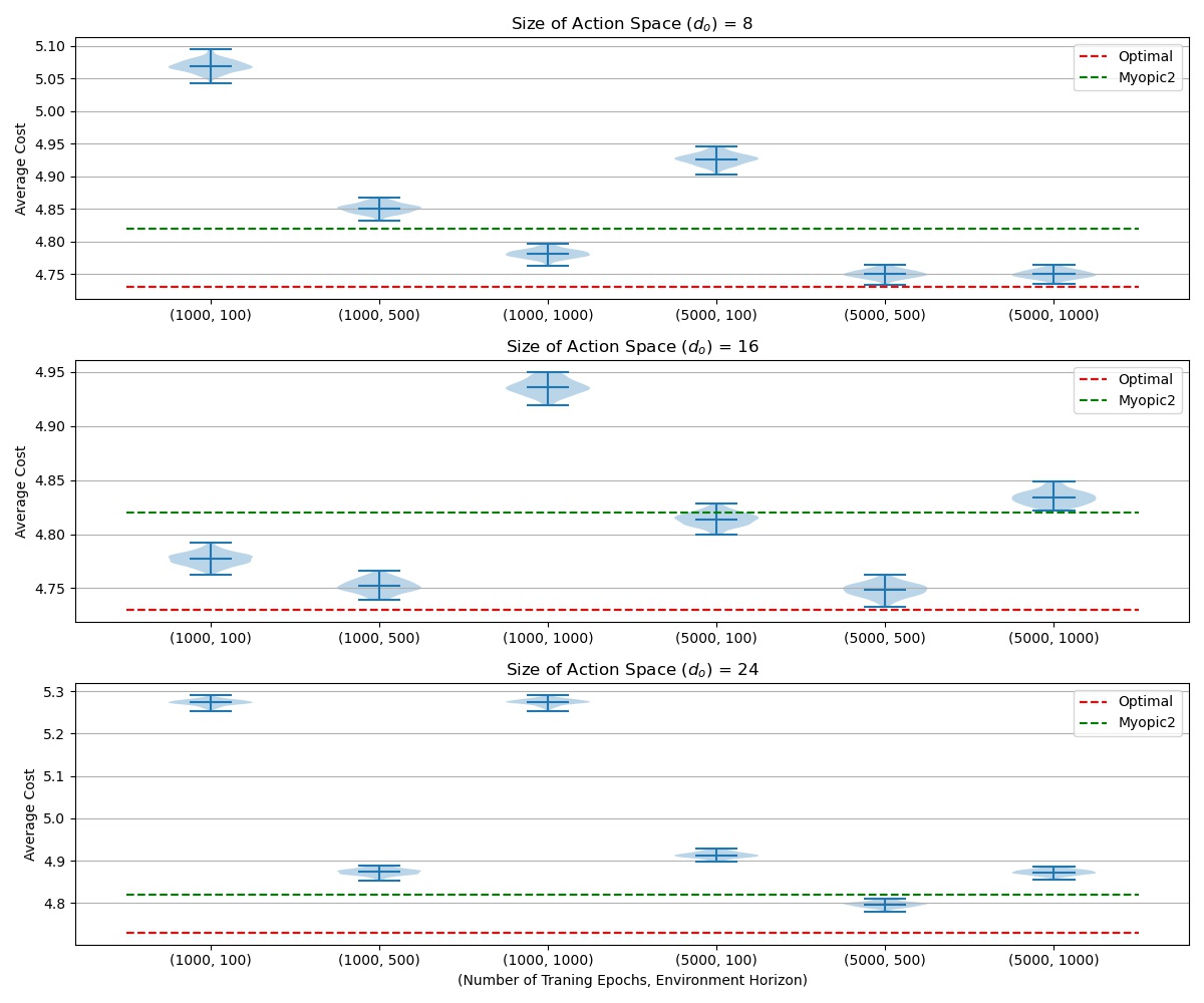
In this section, we evaluate the performance of trained models on 100 different environments generated using 100 different seeds. We set the horizon of the evaluation environment to be one million periods and report the average cost per period of the system. We compare the performance of the trained models with that of the optimal solution and Myopic2 policy for the Easy and Medium problems, and only the Myopic2 for the Hard problem.

We consider the impact of three different variables on the performance of trained ES agents:

Number of training epochs
Duration of the environment horizon: the environment horizon determines the accuracy of the performance of an ES individual. The lower horizon lenght may result in a noisy estimate of the individual’s performance. While, longer horizon length result in more accurate estimates of the individuals performance at the cost of increased comutational time.
Size of the output space of the neural network: The output dimensions of our policy architechtures are calculated using the upper bound introduced in Zipkin (2008) obtained using the Standard-Vector-Base-Stock policy ($d^{svbs}$). We set the output dimension of the neural networks to be $d^{svbs}$, $2 d^{svbs}$, and $3d^{svbs}$.

Lost sales problems with Poisson demand distribution

Medium difficulty problem

The medium difficulty problem that we consider here is presented in Zipkin (2008). The Myopic2 policy reaches 1.9% of the optimal average reward per episode which is the highest percentage gap for the problems considered there for the Myopic2. Gijsbrechts (2019) reports that Asynchronous Advantage Actor Critic (A3C) algorithm can train policies that are 6.7% away from optimal solution. A3C performance is also the worst for this problem amongst the problems considered in Zipkin (2008).

Conclusions

In this post, we show how to train neural networks that order new products for the lost sales problem based on the current state of the system using ES. We demonstrate that ES has several advantages over the Reinforcement Learning methods in learning agents for solving the lost sales problem. We summeize these advantages as follows:

ES can train agents that perform near-optimal with a significantly lower computational budget in compariosn to the model-free DRL methods.
ES can achieve these results without the need for hyper-parameter optimization.
The gradient-free nature of the ES enbales us to optmize the obejctive function of the problem directly. Hence, there is no need for reward-shaping and defining different loss functions using ES.
ES can achieve near optimal solutions with significantly smaller neural networks in comparison to the neural network achitechtures reported in the literature.

Note that our objective in this study is not to achieve the best performing trained models, rather to show that ES is able to reach near-optimal solutions in a efficient way without need for hyper-parameter optimization. One may increase the population size of the ES (which is quite low in our experiments) or increase the horizon of the environments during the training phase to obtain better policies. Alteratively, one may use the neural network parameters found by the ES as an starting point for the classical RL methods such as Q-Learning to further tune the parameters of the neural nets to obtain better results with significantly lower computtion time.

Citation

If you find this work useful, please cite it as:

@article{Manaf2021LostSales, title = “Evolution Strategies as an alternative to Reinforcement Learning for Solving the Lost Sales Problem”, author = “Manafzadeh Dizbin, Nima, Basten, Rob”, journal = “nimaman.github.io”, year = “2021”, url = "" }